Simplified parametric modeling to predict vibration attenuation provided by on-grade slabs

ABSTRACT

When measured vibration amplitudes at the proposed site for a highly sensitive facility exceed the maximum allowable for the sensitive equipment, mitigation measures must be integrated into the design that will reduce the vibration amplitudes to meet the requirements. Past studies have shown that thick concrete slabs supported on a well-engineered subgrade can effectively reduce ground borne vibrations at certain frequencies. Predicting the vibration performance of a new slab-on-grade can be a significant challenge, however, as the performance is highly dependent upon the site soil conditions and nature of the vibration sources impacting the location, as well as structural characteristics. Large and detailed three-dimensional finite element analysis models of the site conditions and proposed structure are often used for this type of assessment, however development of such a model requires significant time and cost to develop accurately. This paper discusses a proposed alternative simplified parametric modeling technique using two-dimensional plane strain modeling. This technique can be utilized in combination with real-world data to predict the relative benefit of various slab thicknesses and design features such as structural breaks. This includes multiple comparisons between predicted results using this methodology and field measurement results.

PDF Download

1. INTRODUCTION

The design of a facility intended to house vibration-sensitive equipment often begins with a vibration survey at the proposed location. Ambient and transient-induced vibration amplitudes measured at the site, whether it is an undeveloped greenfield or an existing building that is to be renovated, are an important indicator of the suitability of the location for sensitive instruments. However, amplitudes measured as part of the site survey do not necessarily represent the expected vibration environment once the facility is completed. The addition of a building or modification of an existing building structure can have a significant impact on the site vibration environment – a phenomenon called the “building effect” that has been well documented in past studies.[1,2,3] For an on-grade floor in a building without a basement, the building effect is generally due to the mass and stiffening effects of the building frame, footings, and slab-on-grade floor, as well as the distance the vibrations must travel through the slab. The subset of these factors that are related to the slab-on-grade design specifically, which we will call the “slab effect”, will be the focus of this paper. Specifically, we will discuss a proposed parametric modeling approach that can help to assess the relative benefits of various slab-on-grade details with regard to vibration attenuation.

______________________________

2. PLANE STRAIN MODELING

Three-dimensional finite element analysis of vibration propagation in soils and soil-structure interaction is common, particularly for seismic analysis. These models can be very sophisticated and allow for highly detailed predictions of how a particular soil profile and structure might respond to dynamic excitation. However, these models are generally very large and complex, making them very time consuming to construct and manipulate. Dynamic analysis using large soil models can sometimes require solver run times of many hours – even at modern processing speeds. This can make the number of model iterations that are often required to study certain design variables very time consuming. On projects with limited budgets and tight schedules, this is often not practical.

In order to approximate the anticipated slab effect, we will instead utilize a two-dimensional plane strain finite element model. A plane strain model, in essence, represents a slice of unit thickness through the half-space being modeled. At the element and nodal level, the model is assumed to be constrained on the near plane and the far plane bounding the slice, such that rigid support is provided into and out of the plane of the paper, while leaving the nodes and elements free to deform vertically and horizontally within the plane. Further, it is assumed that all deformation is displacement, and rotation is not provided. A half-space can be modeled using far fewer elements and nodes than a three-dimensional model, significantly reducing modeling time.

The intended use of this model is for parametric properties, rather than attempt to make specific predictions for a specific site. In other words, we will be able to compare the effects a certain design detail (such as a joint in the slab) or examine how performance varies with a dependent variable such as slab thickness. The objective is to develop generalities about the expected slab effect.

2.1. Model Parameters

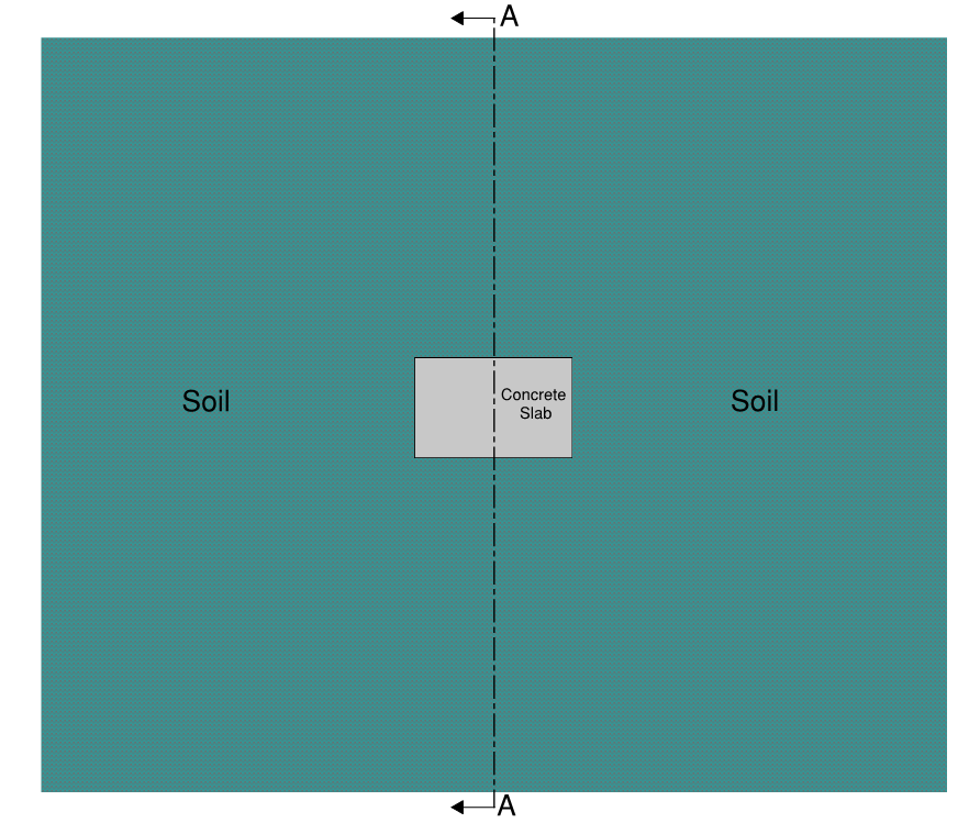
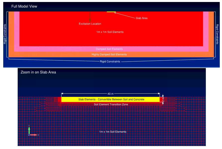
A plane strain model can be constructed to represent a concrete slab surrounded by contiguous soil. A schematic plan view of the scenario modeled is shown in Figure 1. Section A-A shown in this schematic is represented in the plain strain model shown in Figure 2.

Key features of this model include the following:

• The following material properties were used for the soil and concrete:

• Typical soil quadrilateral plane strain soil elements are 1m x 1m, with a transition zone of progressively smaller elements when approaching the slab area. Given that the wavelength of vibration in clay silt with the properties above is 4 meters at 50 Hz, this allowed the model to adequately represent vibration up to this frequency while maintaining at least 4 nodes per wavelength.
• Elements in the slab area are 125mm x 25mm (aspect ratio 5:1). These elements are designed to be easily changed between soil and concrete to represent conditions between greenfield (100% soil) and concrete slabs up to 2 meters thick and 40 meters wide.
• A material damping ratio of 0.1 was used for the soil and 0.03 for the concrete.
• The extent of “normal” soil is 850m wide x 160m deep, and beyond that is 50m of highly damped soil in two layers on all both vertical sides and the bottom. The intent of the highly damped soil is to provide an anechoic boundary along the sides and bottom. A damping ratio of 0.6 was used for the inner 25m of highly damped soil, and 1.0 for the outer 25m layer of highly damped soil.

2.2. Analysis Procedure

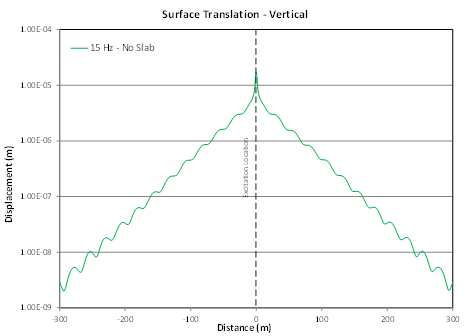
The model was excited with a point load using a dynamic sweep in increments of 1 Hz between 5 and 50 Hz. It should be noted that, in the plane strain representation, point loads applied to this model effectively represent a line load. The sweep was applied at various locations in the model, and the resulting displacement of the surface nodes across the model was extracted for each frequency. The load point was generally kept at least 20 meters away from the edge of the slab, to represent farfield loading at most frequencies of concern, although nearfield loading will also be explored. Figure 3 shows an example plot of predicted displacement of the surface level nodes for a greenfield case at 15 Hz.

The slab effect was modeled based on the relative response between two different model cases. This is important since many of the variables and assumptions described above are held constant across the two cases. This means that it is less critical that variables such as damping, which can be extremely difficult to predict, accurately match the conditions in questions.

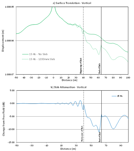
Figure 4a shows the same predicted greenfield surface response as in Figure 3 compared to a second curve showing the predicted displacement of the same nodes with a 1200mm slab added 40 meters away from the load point. The plot has been zoomed into the slab region for clarity. Note that the predicted response in the areas away from the slab is identical in the two cases, as expected. The predicted responses of the slab nodes are different. The ratio between the two responses at each location, expressed in decibels, can be used to represent the slab effect at each location – as shown in Figure 4b. Negative values in these curves represent attenuation, or “insertion loss” provided by the slab compared to the greenfield (or another baseline) case. Note that the model results imply some slab effect for the soil nodes in the vicinity of the slab as well – with a “shadow” zone on the far (right) side of the slab relative to the loading, and a reflection or interference zone on the near (left) side.

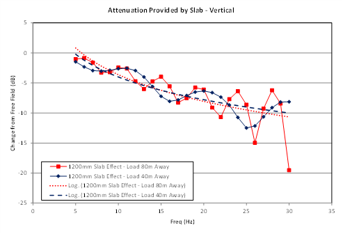
We evaluated the average insertion loss of several nodes across the portion of the slab of interest at each frequency, rather than selecting a single node for analysis. This helps to reduce the influence of potential mathematical artifacts and anomalies caused by the simplified model – including point loading, which has zero width and is not representative of real vibration sources, as well as reflections and phase differences that might be overemphasized in the simplified model conditions. This allows the predicted insertion loss of a slab to be expressed as a single value at each excitation frequency. For example, Figure 5 shows the predicted attenuation provided by the slab as a function of frequency using two different excitation locations – 40 and 80 meters away from the edge of the slab. The predicted insertion loss as a function of frequency changes somewhat depending upon the excitation location relative to the slab, with “oscillations” that show increased deviation from one another with increasing frequency. Importantly, the predicted attenuation in each case oscillates around a nearly identical trendline, and this trendline will be used to determine the predicted slab effect.

3. MODEL VALIDATION

In order to better understand the accuracy, and limitations, of this model for use in parametric studies, we modeled a few cases for comparison to known or measured results.

3.1. Rayleigh Wave Propagation

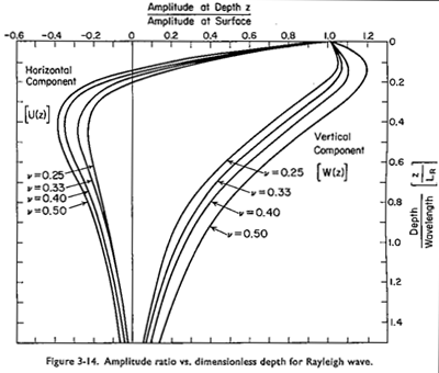
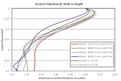
Ground vibration that is typically of most concern for sensitive buildings propagates in the form of Rayleigh (surface) waves. Therefore, a sweep load applied to the plane strain model should approximate Rayleigh wave propagation reasonably well. Figure 6 shows a plot of the expected relative amplitudes as a function of wavelength and depth beneath the surface in Rayleigh wave propagation.[4] Curves are shown for various values of ν, the Poisson’s Ratio of the soil. Figure 7 shows an example of the model’s predicted response of greenfield conditions as a function of depth for vertical vibration at 10 Hz – a frequency chosen somewhat arbitrarily for illustration purposes. Predicted results are shown at various distances away from the load point. These amplitudes are shown in comparison with the expected amplitude ratio as a function of depth for Poisson’s Ratios of 0.25 and 0.33 in Figure 6 – since our model assumed a ν of 0.3. There is some variation in the predicted results depending upon the proximity to the load point, and the agreement with the published curves is not exact. However, each curve predicted by the model has a characteristic shape that is quite similar to the theoretical curves, which is a good indication that the model is representing Rayleigh wave propagation well enough for the purposes of a parametric model.

3.2. Comparisons to Measured Data

Another way to validate the plane strain model is to compare the predicted slab insertion loss to measured data that represents the real attenuation provided by a slab. Reliably extracting the slab effect from real world measured data is very difficult, due to the number of other variables involved that are inherently uncontrollable. Real conditions are also likely to introduce far more variation than in our idealized, simplified model – and therefore a precise match between measured and modeled performance is not expected. However, if the general trends identified in our model match some general trends evident in measured data, this can help to validate the modeling approach. Just as importantly, it can also help to identify its limitations.

_____________________________

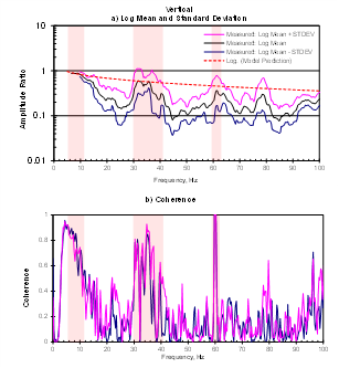
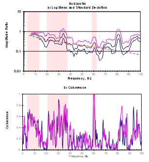
Figure 8 shows the measured slab effect of a 300mm slab in the vertical and horizontal directions – a case that has been summarized in detail in a previous study.[2] The plots show a statistical summary (log mean +/- standard deviation) of the ratio of amplitudes measured on and off the slab due to ambient excitation, as well as the coherence of the measured data between the two locations. Note that, in this case, the coherence refers to the similarity of the vibrations measured at the two locations, rather than the quality of a transfer function.^[3] The dashed red line in both plots shows the insertion loss at the middle of a 300mm slab of similar dimension predicted by our model.

The predicted vertical insertion loss only shows close agreement with the measured insertion loss in certain frequency ranges, which are indicated in pink shaded rectangles in the plots. These frequency ranges align with the range in which the coherence of the measured data was fairly high (> ~0.5). This implies that the model does provide a reasonably accurate of the slab effect, but only in frequency ranges where vibrations measured on and off the slab are similar (coherent), probably due to the same source. The measured results deviate significantly from the model in frequency ranges where the “source” is more diffuse, without directionality or an orderly phase relationship.

The horizontal results also show good agreement with the predicted trendline from our model, up to around 70 Hz, with the exception of results around 30 to 40 Hz where a large hump in the measured spectrum is not present in the trend predicted by the model. In this case, even the lower coherence results match well with the model prediction.

_{³It might be argued that the meanings of “similarity” and “quality” of the FRF are virtually identical.}

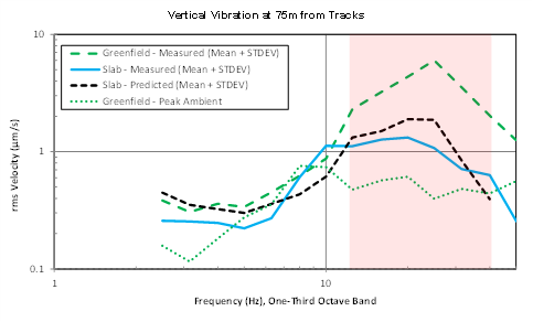
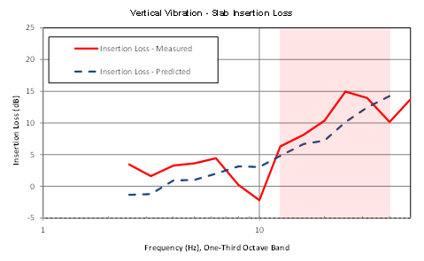
In another case measurements were conducted at the same location roughly three years apart: before and after the construction of a 900mm slab and surrounding building structure. Measurements in both conditions were conducted while trains passed on a nearby rail line approximately 75 meters away. Figure 9 shows vertical vibration amplitudes measured at this location, in RMS velocity using one-third octave bandwidth. Multiple train passages were measured in both conditions, and the log mean+standard deviation of the peak-hold amplitudes measured across all train passages are used to represent the amplitudes for both cases. The pink shaded areas represent the areas in which the peak vibration amplitudes measured due to the trains exceeded the peak ambient levels. The train can be considered to have a significant vibration impact only at frequencies where the train-induced vibration significantly exceeds the peak ambient vibration (i.e. f ≥ 10 Hz).

The predicted vibration amplitude, which was calculated by applying the predicted insertion loss from our model to the measured greenfield amplitudes is shown in Figure 9 as well, along with the predicted and measured insertion loss of the building. Notably, the predicted and measured insertion loss curves align well in the shaded areas – though the model consistently underpredicts the insertion loss.

Underprediction from the model is expected in this case. Since the entire building structure was completed at the time of measurements, the difference in measured amplitudes would more accurately be considered to represent the entire building effect, rather than just the slab effect. The difference between measured and predicted in this case could be considered to represent the additional attenuation from factors not included in our model, such as added stiffness provided by the superstructure, foundation, etc. Of course, it also must be noted that the data used for this comparison did not utilize an identical excitation. While the trains and conditions in each case were similar, even small changes in the track conditions over the course of the time required to construct the building, or differences in the specific trains measured, could significantly alter the measured amplitudes.

The frequency range where train vibration significantly exceeds the ambient is analogous to the high coherence regions in Figure 6 above. When vibration amplitudes are dominated by a determinant source – similar to the modeling approach of applying a load at a single distinct location – the slab effect predicted by the model appears to agree well with measured data. This may imply that the model is more accurate for predicting the attenuation of a known, nearby source, rather than of more random, non-directional sources. Coherent vibration in our measurements could also be more heavily dominated by the Rayleigh wave vibration that is simulated in our model.

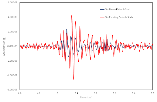
In another case, we measured the vibration response of two different slabs of different thicknesses in the same building at the same time. The vibration source in this case was a guillotine machine used for cutting large stacks of paper, which was in the same building as the measurement locations. Vibration was measured simultaneously on two different slabs: a 125mm slab-on-grade supported on soft clay, as well as on a 1000mm thick slab over improved subgrade over the same soft clay. The measurement locations on both slabs were around 20 meters away from the guillotine, roughly 5 meters apart from one another. The guillotine was located on a 125mm slab that was contiguous with the slabs being measured. The guillotine generated impulsive vibration with each cut, generating waveforms similar to those shown in Figure 10 at the two locations.

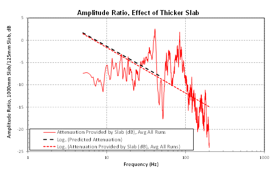
The difference in amplitude between these two locations as a function of frequency, representing the added attenuation provided by the thicker slab, is shown in the red trace in Figure 11. This plot also shows the difference in amplitudes between a 125mm and 1000mm slab predicted by our model, shown as a black dashed line. In this case, results from the model were generated using an excitation point on the slab, rather than on the soil in the farfield, to attempt to represent the actual measured case.

In this case the predicted and measured results diverge at most frequencies. While there is less than 0.5 dB of difference between the logarithmic fit of the full measured dataset – shown as a red dashed line – and the predicted slab effect – shown in the black dashed line, the low quality (low-R) of the fit indicates that this may be more coincidental than meaningful. The model significantly underpredicts the slab effect at very low frequencies. This could be due to the impulsive nature of the source, which is effectively a point load, compared to the sinusoidal line loading used in the model. The two-dimensional model also may not be accurately capturing the effect of the stiffness and mass of the larger slab. This could be particularly important in a case such as this, where the thick slab is likely in the nearfield at low frequencies. At higher frequencies, the measured slab effect is clearly impacted by resonances of the two slabs measured, or differences in subgrade resonances. This results in a large amount of attenuation in some frequencies – including the frequencies at which the guillotine generated the highest amplitudes – but minimal to no attenuation at other adjacent frequencies. These types of resonances would not be captured in our half-space model. These data illustrate that a simplified model will not capture all of the variables that determine the precise vibration performance of a slab-on-grade – it is more appropriate to limit this modeling to identifying trends via parametric studies. It may also indicate that vibration propagation within buildings is too complicated to be accurately represented in a model like this.

4. CONCLUSIONS AND NEXT STEPS

The results from this study indicate that the slab effect trends predicted by the plane strain model agree reasonably well with expected performance, based on published data and past measurement studies. However, the examples illustrate that certain site-specific characteristics such as resonances and other details are not necessarily captured in the simplified model, and therefore the model should be reserved only for identifying general trends rather than precise prediction of vibration amplitudes.

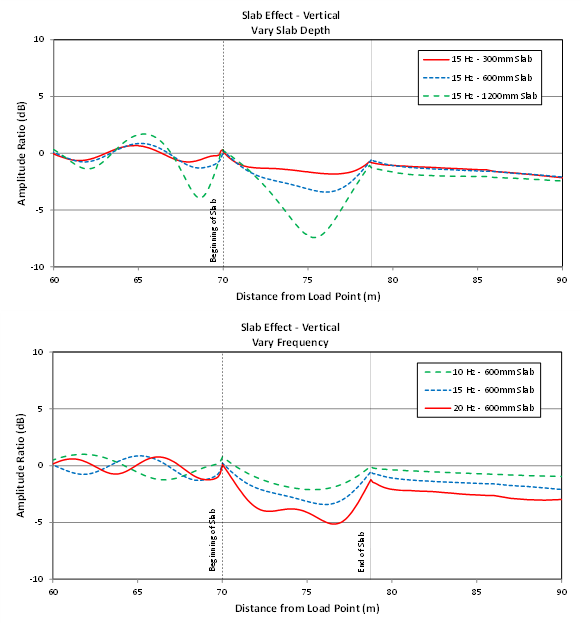
Future studies will utilize this model to examine various trends related to slab-on-grade design and how it impacts vibration attenuation. The model allows for certain variables to be examined in isolation in a way that is generally not feasible using field measurements alone. Figure 12 illustrates a few of the variables that will be explored in further depth in future studies. These include:

• Slab effect as a function of frequency and slab thickness, including how “receiver” position on the slab relative to the source impacts the insertion loss
• The impacts of slabs-on-grade on surface vibration beyond the slab—an apparent “shadow effect” that appears to vary with frequency, but less so with slab thickness
• Reflections at the leading edge of the slab that appear to vary more with slab thickness than with frequency.

In addition, parametric modeling will be used to further evaluate the slab effect in the vertical versus horizontal directions, as well as other common variables such as joints and islands within slabs, below-grade slabs, and soil/subgrade conditions. Many of these factors have been studied previously, primarily using measurement data. Parametric modeling will be used to further explore trends and generalities that have been found via measurements, which can in turn lead to more informed decisions in the design of future vibration-sensitive buildings.

5. REFERENCES

1. Amick, H, Xu, T., & Gendreau, M. The Role of Buildings and Slabs-on-Grade in the Suppression of Low-Amplitude Ambient Ground Vibrations. Proceedings of the 11th International Conference on Soil Dynamics & Earthquake Engineering (11th ICSDEE) & the 3rd International Conference on Earthquake Geotechnical Engineering (3rd ICEGE), Berkeley, CA, pp. 877-881. (7-9 January 2004).
2. H. Amick, N. Wongprasert, J. Montgomery, P. Haswell, D. Lynch. An experimental study of vibration attenuation performance of several on-grade slab configurations. Proceedings of SPIE Conference 5933: Buildings for Nanoscale Research and Beyond San Diego, CA. (31 Jul 2005 to 1 Aug 20)
3. Xiong, B., Amick, H., Gendreau, M. The Effect of Buildings on Ground Vibration Propagation. Proceedings from NoiseCon 2007, Reno NV. (2007 October 22-24).
4. Richart, F. E., Hall, J. R., and Woods, R. D., Vibration of Soil and Foundations, Prentice-Hall, Englewood Cliffs, NJ, 1969.