Abstract
The design of vibration-sensitive advanced technology facilities generally involves considerable attention to structural and mechanical aspects. In most cases, the vibration control measures contribute significantly to a facility’s cost. The selection of a vibration criterion for use in design is an important step in the design process. Many process equipment manufacturers have provided tool-specific criteria, and the literature contains several forms of “generic” criteria. Unfortunately, there is no standardization in either tool-specific or generic criteria, and considerable confusion can arise. Often the confusion is associated with the forms of data representation being used. This paper first reviews some of the relevant fundamentals of signal processing, then uses experimental data to develop a tool-specific vibration criterion for an optical microscope. Two dissimilar approaches to generic criteria are discussed and their signal processing requirements are examined. They are compared with a manufacturer’s published vibration criteria for a projection aligner. Recommendations are given for future development of tool-specific criteria.
Introduction
Many processes involved in advanced technology applications are highly sensitive to vibrations. Among these processes are precision metrology, high-energy physics, long-beam-path laser applications, biotechnology research, and the R&D and production of semiconductors. Typically, the work carried out in these facilities requires environmental conditions more sophisticated than those provided by buildings intended for conventional occupancy. In many cases, vibrations are of concern. During the design of such facilities, architects, structural and mechanical engineers, and vibration consultants employ measures to reduce the severity of vibrations to which vibration-sensitive process equipment (“tools”) is exposed. These measures include definition of design vibration criteria and various forms of engineering analysis intended to assess and limit vibrations.
In general, vibrations pose a problem for tools because they generate internal relative motion along a beam path that either blurs an optical image or causes an electron beam to deviate from its intended path. The ultimate objective of vibration control design should be to limit the extent of internal disturbances of a tool by limiting the floor vibrations where it will be installed.
Several types of vibrations are present in advanced technology facilities, and each should be given consideration during design or evaluation. The nature of each type of vibration should be considered when selecting the form in which the criteria are defined and the data are analyzed. The remainder of this paper will be concerned with vibration data representation and vibration criteria for tools and facility design. Recommendations will be given regarding the types of data that would be most useful to designers when presented in tool-specific criteria.
Vibration Data Representation
Discussion of vibration criteria or vibration analysis can be addressed in three parts: (1) the analytical domain to be used for data representation (time domain vs. frequency domain); (2) the metric to be used (displacement vs. velocity vs. acceleration); and (3) the statistical form, generally a choice between instantaneous and energy-averaged amplitude.
It is very important that the domain, metric and statistical form of a criterion and corresponding analytical methods should lend themselves to assessment of both analytical data (from predictive structural models) and measured data from a site or building. To do this they should provide a meaningful basis for the characterization of a vibration environment. The discussions that follow will address some of the analytical and signal processing aspects of data representation that must be considered in selection of a methodology.
Time vs. Frequency Domain
Vibration displacement, velocity or acceleration can be stated in either time or frequency domain. Time domain data have been defined as “equivalent representations of physical motion, wherein motion is quantified as a set of amplitudes as a function of time.”1 Frequency domain data have been defined in a similar manner, except “as a set of amplitudes as a function of frequency.”1 It is common to refer to time domain data as a “time history” and frequency data as a “spectrum.”
In the time domain, one can work with either instantaneous amplitude or an average such as root-mean-square (rms). Use of instantaneous amplitude requires consideration of the algebraic sign of the amplitude with respect to the “at-rest” position. The severity of instantaneous amplitude can be characterized by a maximum value over some period of time, either as 0-to-peak (the maximum absolute value) or peak-to-peak (the absolute sum of positive and negative peak amplitudes1).
In frequency-domain analysis, time-domain data are transformed in some manner to spectra. Spectra are defined by their frequency bandwidth and, in the context of vibration-sensitive facilities, are most commonly stated as (1) constant bandwidth (a.k.a. narrowband), (2) one-third-octave (a.k.a. proportional or percentage) bandwidth, or (3) spectral density. When working with measured vibrations, constant bandwidth and density spectra are typically obtained using Fast Fourier Transform (FFT) analysis, and one-third-octave band spectra are obtained by using either parallel filtering or a synthesis based on FFT analysis. All have evolved from the digital signal processing requirements of acoustics, physics, electrical engineering, and mechanical engineering. There is a large body of literature associated with spectral analysis of random and tonal vibrations. Time-tested methodologies exist for characterizing vibration signals ranging from stationary or periodic to impulse, shock, and other transients.2, 3
Types of Data Signals
Measured vibration data are commonly acquired as analog time history signals produced by acceleration or velocity transducers such as accelerometers or seismometers, respectively. From a data analysis viewpoint, time history signals are divided into two broad categories, each with two subcategories, as follows:4
1. Deterministic data signals: (a) steady-state signals; (b) transient signals.
2. Random data signals: (a) stationary signals; (b) nonstationary signals.
Deterministic Data: Deterministic data signals are those for which one can, in theory, predict future time history values of the signal (within reasonable error) based upon a knowledge of the applicable physics or past observations of the signal.4 A periodic signal is one that repeats itself after a constant time interval. The time history of the vibrations generated by one rotary mechanical system can take the form of either a single frequency (a pure tone) corresponding to the shaft rotation rate or that of a series of harmonics, the frequencies of which are integer multiples of the shaft rate. In the presence of a collection of independent (unsynchronized) periodic sources (such as the mechanical plant in a “fab”—a microelectronics fabrication facility), the collective time history may not be rigorously periodic—in this case it is referred to as “almost periodic.”4 “Transient” deterministic data signals are those that begin and end within a reasonable measurement time interval; these can include those from equipment startup and some types of well-controlled impacts.
Random Data: Random vibrations are broadly defined as those that are not deterministic, that is, where it is not theoretically feasible to predict future time history values based upon a knowledge of the applicable physics or past observations.4 In the time domain the amplitude—including the peak amplitude—is random. There is no periodicity. Random motion is typically characterized by an average amplitude, the most common of which is the rms value discussed above.5 In addition, there is no frequency directly associated with random vibration and a spectrum must be used to define the frequency content.
If the average properties of the signals are time invariant, such random data are said to be “stationary.” If the average properties of random signals vary with time, the signals are said to be “nonstationary.”4 (An example of nonstationary random ground vibrations would be those associated with the passage of a train.)
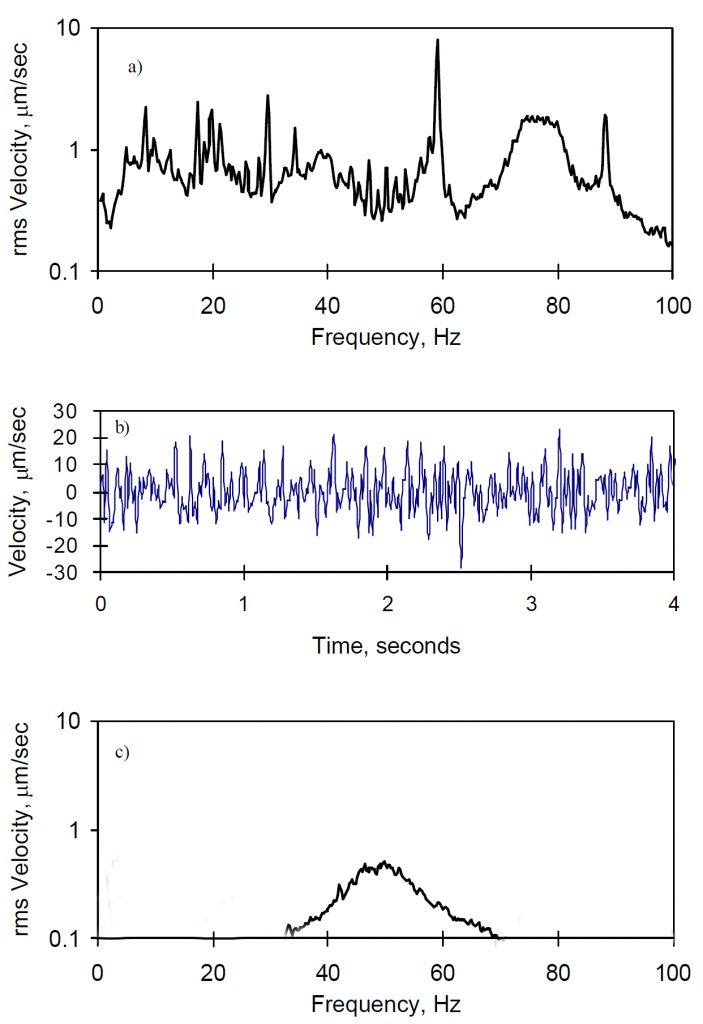
The Nature of Floor Vibrations: (a) shows a fairly typical constant-bandwidth spectrum of vibrations measured on the floor of a 20 year old fab; (b) shows a segment of the associated time-history. The spectrum has single-frequency (“tonal”) components (the sharp peaks), but the time history is dominated by the random vibration components and exhibits little or no periodicity. (c) shows a spectrum—almost entirely random—measured soon after startup in a facility now only a few years old. Floor vibrations in virtually any operational advanced-technology building will be a similar complex mixture of random and almost-periodic tonal signals, described below.
- The most common sources of periodic vibrations are constant-speed rotating equipment, such as that typically found in the mechanical plants of these facilities. If there are n pieces of rotating equipment, there will be n tonal components of varying amplitudes. The collective result of all of these sources is most likely almost periodic.
- The ground supporting the structure is vibrating (due to traffic and other external sources) and this can propagate into the building. These vibrations are inherently random and usually composed of both stationary and transient components. (Occasionally, a neighboring facility might contribute periodic vibrations from its own mechanical plant. It should be considered in the previous category.)
- People walking on the floors generate impact loading. Typically, these repeated impact loads generate vibrations that start with a peak amplitude followed by a decay, of which the fundamental resonance frequency of the floor system is the primary component.
- If large air ducts are supported from building components, the air turbulence within them may generate random dynamic forces that are transferred to their attachment points. There can be many such attachment points.
- If large process piping is supported from building components, the liquid turbulence within them will generate random dynamic forces. Each ducting and/or piping connection point (e.g., hanger rod) becomes a loading point at which a random force function is applied.
- Low-frequency airborne acoustic noise at the high levels commonly encountered in fabs represents random air pressure fluctuations which can excite structural components, which can include walls, tables and floors as well as tools themselves.
Instantaneous vs. Time Averaged Representation
It is often convenient to represent an oscillating signal in a form that does not involve positive and negative amplitude. One cannot generally use a time-varying average, as commonly defined, because in many cases the average of an oscillating signal is zero. We use the average energy, or root-mean-square (rms), defined in the following equation, since it is based upon the square of the amplitude, which is always positive.
Generally, this process is carried out electronically by an analyzer of some sort. The integration period T can be set as appropriate to the analysis. If the average is taken over a short period, such as a second, the moving energy average can be plotted as a function of time. If the average is taken over a significant time period, then it is quite common to refer to this as the equivalent level, Leq.

For most purposes, a sinusoid can be completely characterized by its amplitude and its frequency. (Generally the phase is of little practical importance in the contexts being discussed.) Since steady-state deterministic vibrations are commonly made up of sinusoids and are generally either periodic or almost periodic, the peak is subject to systematic repetition, although there may be a significant interval between repetitions. Thus, it is not unreasonable here to characterize the severity of the vibrations by means of the overall peak or peak-to-peak amplitude.
Unfortunately, the situation regarding non-deterministic vibrations is not as straightforward. It is common in random vibration theory to speak of a family or ensemble of time histories. The property of ergodicity dictates that for stationary vibrations the energy average (rms) amplitudes of all members of the ensemble will be identical.6 This repeatability of the average amplitude—as opposed to the nonrepeatability of the peak amplitude—is a major reason that random vibrations are characterized by averages. This thinking can also be extended to situations involving deterministic vibrations mixed with a significant level of random vibrations.
Peak vs. Time-Averaged Criteria
The universal application of a maximum amplitude—as opposed to some sort of statistical representation like the energy average—has several shortcomings, which follow from the previous discussion. They relate to the following:
- statistical rarity of the instantaneous peak;
- response associated with events of very short duration; and
- definition of “peak-to-peak”.
Statistical rarity of the instantaneous peak. How well does the instantaneous peak represent the environment being considered? If we are dealing with vibrations made up of a limited number of tonal components or the vibrations associated with the decay of a footfall impact response, the definition of an instantaneous peak is relatively meaningful. However, if we are dealing with a vibration environment in which random vibrations predominate (typical in a site assessment, common in a fab) the peak amplitude will be dependent upon the sample duration. Probability theory suggests that the longer one waits when evaluating a stationary random environment (or the larger the sample duration), the larger will be the maximum amplitude. This is true in either the time or frequency domain. However, if one uses energy averaged representation (such as rms), then the amplitude of a stationary random signal will be relatively constant.
Response associated with events of very short duration. An instantaneous peak (in time domain) may define the maximum amplitude over a period of time but may not contribute significantly to an energy average. In this condition, does the peak necessarily represent how a tool will respond? How does one establish for a particular tool the threshold between steady-state response and shock response? Available data are inadequate to develop a general answer, but many believe that rms averaging provides a more appropriate representation of how a tool will respond in most cases, depending upon the averaging time involved. In one particular case involving a laboratory being designed for high-energy-physics research, the client’s project director—a highly competent physicist—insisted that instantaneous representation not be used, because his studies had indicated that vibrations must be of significant amplitude when “integrated over a period of at least one second” (which corresponds to an rms averaging time T of one second) in order to affect his apparatus.
It would be too simplistic to suggest that rms amplitude is appropriate for all situations, particularly if the averaging time were long. There can be cases where an instrument could be excited by a single pulse in a support vibration, whereas other systems might require a certain duration of sustained duration. Researchers concerned with the effects of peaks devised a metric called the “crest factor,” the ratio of peak value to rms value. For a simple sinusoidal vibration, the crest factor is 1.414. As the crest factor increases, the analytical scenario moves from steady-state to shock. A low crest factor implies that the vibration is reasonably well characterized by the rms value; a high crest factor suggests that the vibration may be better characterized by the peak value or a shorter rms averaging time. The significance of crest factor and averaging time have received considerable study with regard to vibrations affecting humans, but virtually no study with respect to vibration-sensitive tools.7
Definition of “Peak-to-Peak” Value. The American National Standards Institute8 (ANSI) and IES1 provide precise definitions of “peak-to-peak” amplitude. The peak-to-peak amplitude of a sinusoid is two times the peak amplitude. Even for more complex periodic deterministic vibration, it is relatively straightforward to define the peak-to-peak amplitude because the positive and negative maxima are repeated and both are contained within any one period. Random vibration, however, has no periodicity. The positive and negative maxima associated with a stationary signal will probably vary from sample to sample, even if the rms average is constant. Thus, the peak-to-peak amplitude will vary from one time sample to another and may also be a function of sample duration. Thus, peak-to-peak amplitude can be considered representative only in the case of deterministic vibrations.
Assessment of a vibration should be based on a form of data that can be considered representative of that environment. A environment that can be characterized as continuous, steady-state or stationary should be assessed in terms of rms amplitude with defined averaging time, since that is the repeatable quantity. An environment that cannot be characterized in this manner (such as vibrations caused by footfalls, impacts, or certain construction activities) may require special consideration of crest factor or averaging time or the use of actual peak amplitude. Vibrations from transient events, such as train passages, can be considered using an averaging time T that is less than or equal to the duration of the event.
Conversion Between Metrics
It is relatively simple to convert amplitude among units of displacement, velocity and acceleration when dealing with a single sinusoidal waveform (or any other periodic vibration, since periodic vibrations in general can be represented as a sum of sinusoids). At a given frequency f, the ratio of velocity to displacement amplitude is 2f, as is the ratio of acceleration to velocity amplitude. A spectrum is made up of discrete amplitudes (as a function of frequency), each of which represents the portion of the time-domain waveform contributed by a sinusoid at the associated frequency. Since each point on a spectrum represents the amplitude of a sinusoid, it is a simple matter to transform a displacement spectrum to velocity, etc. Thus, it doesn’t matter whether a spectrum (or any other collection of frequency-dependent amplitudes) is presented in units of displacement, velocity, or acceleration, so long as units are adequately stated. No one metric is inherently “better” than another for presenting spectral data.
The Use of Spectra
The domain and metric of criteria and analytical methods must lend themselves appropriately to assessment of the full collection of vibration types found in an advanced technology building. The vibrations at a building site are predominantly random; in an operating fab or laboratory they are random (from the site itself) with a superimposed mix of tonal and random vibrations from mechanical equipment and transient vibrations of various sorts.
An environment made up of steady-state deterministic (tonal) vibrations can be described by stating for each source an amplitude, frequency, and phase along with some scheme to combine effects of the multiple sources. However, Piersol states that unlike steady-state deterministic data, stationary random data must be described by a spectrum.4 Thus, since random vibrations play a significant part in defining the overall vibration environment, spectral representation of that vibration environment is a necessity.
Example—An Optical Microscope
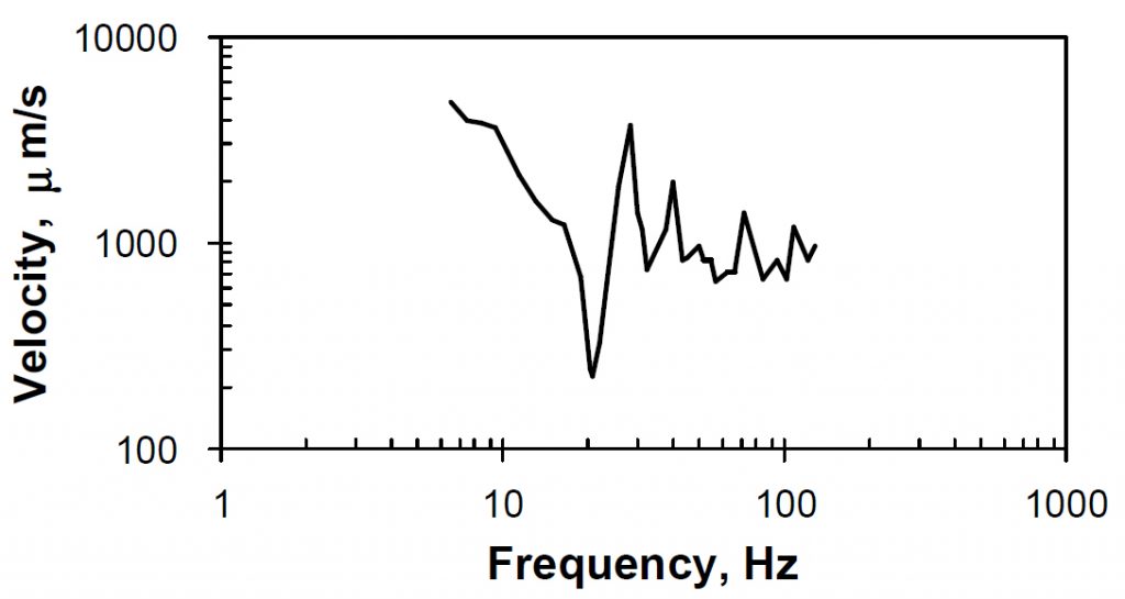
As an example of how spectra can be used to represent measured, tool-specific data, let us examine the results of an experimental study of the vibration sensitivity of a 1000x Nikon microscope used for integrated circuit inspection, working with line widths down to 1 micron. The microscope was placed on a table, the top of which was subjected to sinusoidal excitation at a series of frequencies. (Thus, the results represent vibrations at the base of the microscope, not the floor.) At each frequency, the amplitude was increased until the image of a 1-micron wide line was obliterated. The table-top amplitudes associated with two thresholds were recorded: (1) the first observable onset of vibratory effects and (2) the total loss of image.
shows the curve representing the rms velocity threshold at which side-to-side benchtop motion at which the 1-micron image becomes indistinguishable. One can see the “dip” caused by a resonance at 20 Hz and the “peak” caused by an anti-resonance at 27 Hz. Although this curve is academically instructive, it would be cumbersome to use as a facility design tool. It would be desirable to develop something more simplistic.
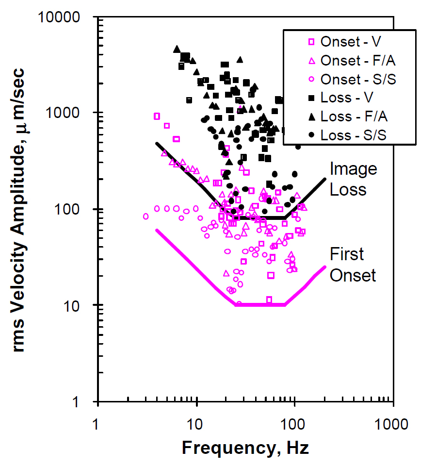
shows the individual data points for these two thresholds. The open symbols show the first visible onset of vibration (either blurring or jiggle, depending upon the frequency); the solid symbols show the amplitude at which the image is entirely lost. On a log-log plot of velocity as a function of frequency, constant displacement can be shown as a line inclined upward to the right. Likewise, acceleration can be shown as a line inclined upward to the left.
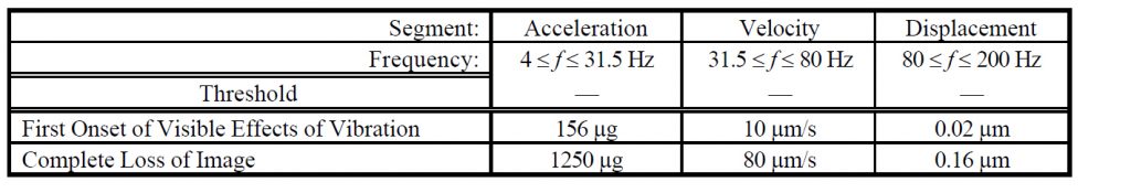
A horizontal line representing a velocity amplitude of 80 µm/s lies just below the lowest two solid data points in . A line inclined downward to the right representing an acceleration of 1250 µg lies just to the left of and below the lower leftmost solid data point. A line representing a displacement amplitude of 0.16 µm lies to the right of and below the data points.
We can define a criterion for image loss that is made up of segments of each curve. Thus, low frequencies (below the lowest resonance) are limited by acceleration, mid-range by velocity and high frequencies by displacement. Another criterion can be constructed for first onset of visible vibration using a segmented curve similar to that for image loss. The one shown in has values one-eighth of those of the image loss curve. summarizes the parameters of the two curves.
The vast majority of vibration consultants use vibration spectra to specify criteria and carry out analysis. The approach is backed up by over two decades of application and study. However, there is at this time no consensus amongst vibration consultants with regard to the type of spectrum to use for design and evaluation (the debate being mostly among the use of one-third-octave band velocity, constant bandwidth velocity or acceleration, and power spectral density).
More significant, however, is the fact that the majority of manufacturers of chip-making tools provide vibration criteria in some frequency-dependent form. Many of these manufacturer-supplied criteria are based upon evaluation of system performance degradation due to controlled vibrational base excitation. Several tool manufacturers treat their vibration criteria as conditions to be met in order to validate their tool warranties. Thus, the facility designer or vibration consultant is somewhat obligated to respect the base-motion requirements published by the individual tool manufacturers.
If the tool installation is correctly executed—i.e., there are no “short circuits”—then a tool’s supports resting on the floor provide the only significant interface between the building system and tool. The tool represents a substructure of the total system; the manufacturers are simply imposing limits on the input to the substructure. Evidence has never been offered—either theoretical or experimental—that there might be tool-structure interaction which would invalidate the concept of a manufacturer imposing environmental limits at the interface between the tool and the building.
Shortcomings of Spectral Representation of Criteria
Spectral representation in any form (whatever the metric or bandwidth) does not necessarily solve all problems encountered during design or evaluation. The users of spectrum-based approaches have long recognized a number of deficiencies or inconsistencies in application. Some of these can be addressed by improvement of analytical approaches, but others simply do not have enough available data for resolution. Two of the more challenging questions we face are the following:
- What are the consequences of simultaneous signals in several different bands? (For example, if the measured spectrum has amplitudes of 6 m/sec (250 in/sec) at both 20 Hz and 40 Hz, do we say that it meets or it exceeds a criterion spectrum that has an amplitude of 6 m/sec at those frequencies?)
- How do we put vibrations due to tones, random excitation and footfall on an equal footing? The relative amplitudes and crest factors of these three categories are extremely sensitive to bandwidth, averaging method, and averaging time. Virtually nothing is known about how the behavior of individual tools varies with these different types of excitations.
Generic Vibration Criteria
If a specific space is being evaluated for a particular tool, one should perform the vibration evaluation using the units and signal processing methods specified by its manufacturer’s installation requirements (assuming that they are known). However, suppose that a facility is in the earliest stages of design, and tools have not yet been selected. It was largely for this situation that the concept of “generic” facility design vibration criteria was first introduced. The initial intent was to characterize the vibration environment that would meet the needs of all tools involved with a particular technology.
Another reason for the popularity of generic criteria deals with the issue of space flexibility: should a fab be designed to meet only the vibration requirements of the tools it will initially house or should it be designed to meet the generic requirements of the full set of tool types that might be used in the future to produce a given line width? The latter choice will in some cases lead to a more expensive structure, because a building meeting a more stringent vibration criterion is generally more expensive. When presented with the question regarding future space utilization, many (but not all) owners opt to pay a higher price for a facility that will “stay current longer.”
Several well-known families of generic criteria are in use. An analytical comparison was presented in 1991 of what are probably the two most popular spectrum-based generic criteria.10 One is defined in terms of one-third octave bandwidth spectra and the other using constant bandwidth spectra. The 1991 study showed that although the criterion families differed conceptually in how they treated tonal versus random vibrations, the use of one in place of the other would not likely lead to a significantly different level of conservatism in design. However, time-domain displacement criteria have been proposed11 which represent a significant philosophical departure. These will be examined and compared with one-third octave band criteria.
One-Third-Octave Band Generic Criteria
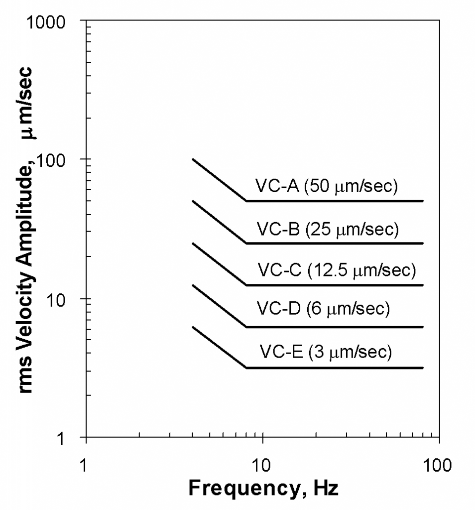
The one-third-octave band rms velocity criteria are given in Appendix C of IES-RP-CC012.1, “Considerations in Clean Room Design,” published by IES in 1993.12 They are illustrated in ; discusses the application of each criterion curve. The reader is referred to Reference 13 for further elaboration. [It should be noted that the criteria in Appendix C are not intended to be the sole basis of design for all facilities. They are given “with the recognition that there are other criterion curves that may have equal validity when adequately defined and used.”12]
The one-third-octave band criteria are generally attributed to Colin G. Gordon and Eric E. Ungar. The earliest published presentations of these criteria were in 1983,14, 15 a decade prior to the appearance of the IES document. They were the product of a review of a large number of tool-specific criteria provided by tool manufacturers. At that time there was little uniformity to the ways in which the tool-specific criteria had been measured or were presented, but many demonstrated frequency dependence in their vibration sensitivity. For this reason, Gordon and Ungar presented their generic criteria in spectrum form. Velocity was chosen over displacement or acceleration, since many of the tool-specific criterion spectra appeared to have as a lower bound a line representing constant velocity as a function of frequency. (In the case of the microscope examined previously, it was desirable to create a criterion that was as “tight” a fit as possible to the measured data. However, many tools are sensitive to vibrations over a broader frequency range, which led to the generalization by Gordon and Ungar using a constant velocity curve between 8 and 80 Hz.)
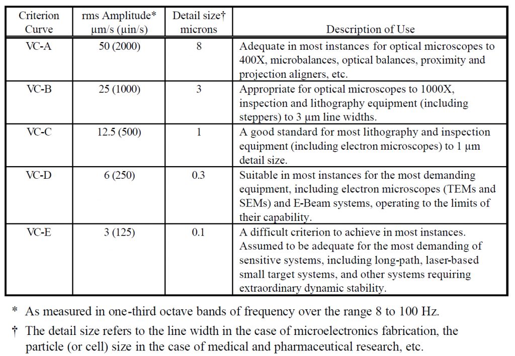
Table 2 relates the various criterion curves to detail size. The logic behind this is similar to that relating clean class and contaminant size to line width: a particle of diameter d may have a much more detrimental effect in the case of a half-micron line with than in the case of a 5 micron line width. For example, suppose that the motion of the stage of an aligner has an amplitude of 0.1 micron. This will be one-fiftieth of the width of a 5 micron line, but only one-tenth the width of a 0.5 micron line. What may be acceptable error for a large line width may be quite unacceptable at much smaller geometries. Although definitive rules for handling this issue have not been published by tool manufacturers, one can argue that as a particular tool or technology type is used for progressively smaller feature sizes, the constraints on vibration must become increasingly stringent. Tool structures are usually linear at the amplitudes under consideration, so the halving of the amplitude of base motion leads to a corresponding halving of the amplitude of beam path motion or other misalignment.
During the years since 1983, the criteria have been presented and discussed in a wide variety of settings, including vibration control literature and conferences,14, ,15 ,16 ,17 a specialty conference of the American Society of Civil Engineers (ASCE),18 a handbook for transportation systems,9 a textbook on construction vibrations,19 a publication of the American Society of Mechanical Engineers (ASME),20 several specialty conferences on vibration-sensitive facilities sponsored by the Society of Photo-optical Instrumentation Engineers (SPIE),10, 13, 21 and in publications and conferences directed toward the semiconductor industry.22, 23
After over a decade of applying these criteria, the author has found that there are several commonly asked questions:
- Why do you show data in velocity units? As pointed out earlier, spectra can be shown in terms of displacement, velocity or acceleration, yet most users of these criteria show them—as well as measured data—only in velocity units. There are two primary reasons. (1) Over most of their defined frequency range each criterion curve has a single value of velocity, so a velocity axis provides the most compact presentation. (2) Because of the nature of a plot of log velocity vs. log frequency, one can tell by visual inspection whether all or a portion of a curve tends more towards displacement, velocity or acceleration simply from which direction it slopes.
- Why do you use logarithmic axes? This practice is recommended by IES-RP-CC024.1, “Measuring and Reporting Vibrations in Microelectronics Facilities.” Vibrations are always present—there is no such thing as a vibration-free environment. A linear vertical axis implies, however, that vibrations of very small amplitude are not significant, which may not be the case. Thus, it is common to present vibration data in logarithmic form so that data can be shown more easily over as many orders of magnitude as necessary.
- What is the significance of one-third octave bands? Aren’t all spectra the same? All spectra are not the same, and this occasionally leads to serious confusion. The difference lies in the bandwidth or frequency range associated with each data point on the spectrum. The bandwidth determines how much vibrational energy is represented by the data point. This becomes significant when evaluating either random vibrations or closely-spaced tonal components. One-third-octave bands are defined by standards in terms of their “center frequencies,” and their bandwidth of each band is defined as 23 percent of the center frequency. Ungar states that “these bands tend to approximate the response bandwidths of equipment, and using them therefore adequately takes into account the effects of closely spaced excitation frequency components.”20 As the name implies, constant bandwidth (or narrowband) spectra have a fixed bandwidth over their frequency range, and different spectrum analyzers offer a variety of choices of bandwidth and frequency range. Density spectra appear similar to those of constant bandwidth, but their bandwidth has been normalized (to 1 Hz) so that measurement bandwidth has no significance when evaluating random vibrations.10
Time-Domain Generic Criteria
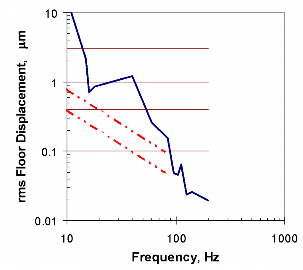
For comparison purposes, let us examine a hypothetical family of peak-to-peak time-domain displacement criteria having four different amplitudes, as defined in . These are assumed to apply to vibrations with frequencies greater than 4 Hz.
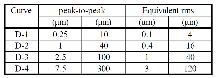
It should be assumed that a time-domain peak-to-peak criterion would be applied to the overall peak amplitude. In the case where the signal is sinusoidal with a single frequency, one can convert from peak-to-peak to rms by dividing by . In this case, the two “Equivalent rms” columns apply. In other cases, such as multiple sinusoids or random vibration, the simple conversion is not appropriate.
Relationship to a Manufacturer’s Specifications
Let us examine an example of how the two forms of generic criteria compare with a manufacturer’s published tool-specific vibration limits. Perkin-Elmer based its limits for the M500 aligner on tests carried out on an airspring-supported shaking table, using sinusoidal excitation in one orthogonal direction at a time. This simulated a “generic” base-support condition which could represent either a floor or a support base. The threshold of acceptable vibration was based upon requirement that “at the wafer plane, mask image motion in either the horizontal or the vertical direction must not exceed 0.1 micron rms.”24
The Perkin-Elmer limits, shown in Figure 5, are defined in terms of rms displacement at frequencies between 2 Hz and 200 Hz (2 orders of magnitude) with amplitudes varying from 0.01 to 10 µm (3 orders of magnitude).
Figure 5 also shows three of the frequency-domain criterion curves from (as transformed into rms displacement spectra) and rms amplitudes corresponding to the four time-domain criterion curves from (assuming single-frequency, sinusoidal excitation).
Comparison with rms Velocity Frequency-Domain Criteria: The tool-specific data lie above VC-A at most frequencies, but fall slightly below it at two frequencies. Criterion VC-B lies below the measured data over the full frequency range of 4 to 80 Hz. This illustrates the concept used by Ungar and Gordon to fit a simple “lower bound” spectrum shape to the data. It forms in part the basis for the generic characterization of VC-A as adequate for projection aligners in general (in ).
In its discussion of the meaning of the limits, Perkin-Elmer infers that the percent error increases as line width decreases. At the time this tool evaluation was carried out (1985), line widths between 3 and 5 microns were typical. As discussed previously, one should safely be able to assume that the tools behave linearly and infer that as line widths decrease the tool would benefit from a more stringent criterion. In two other publications, slightly more conservative approaches have been taken than in : curves VC-B and VC-C have been recommended for aligners working with 3-5 and 1-1.5 micron line widths, respectively.17, 22
Comparison with Peak-to-Peak Time Domain Criterion: Each of the four time-domain criterion amplitudes intersects the Perkin-Elmer curves at some frequency range. None lies entirely below the curves over a significant frequency range without being overly stringent at low frequencies. Criterion D-1 is the most conservative, intersecting in the 50 to 100 Hz range and lying below the Perkin-Elmer curves at all lower frequencies. However, at 10 Hz it is overly stringent by about an order of magnitude. Criterion D-2 intersects the curves in the 30 to 60 Hz range, but lies below all three directional components only at frequencies less than 30 Hz. Criterion D-311 intersects the curves between 8 and 40 Hz, approximating the amplitude of the vertical component, but D-3 lies below the vertical component only at frequencies less than 16 Hz and below all three components only at frequencies less than 8 Hz.
It should be noted that if one limits frequencies to a small enough range, it makes little difference whether one specifies displacement, velocity or acceleration. If one limits the frequency range of interest to a relatively small fraction of the range over which the Perkin-Elmer limits are defined, say 16 to 40 Hz, then one can define rms criteria of 0.6 µm displacement, 60 µm/s velocity, or 600 µg acceleration (these three amplitudes are approximately the same at 16 Hz) and be assured that they will all three lie below the Perkin-Elmer curves in this range. However, if one extends the displacement criterion outside this range, perhaps to assess the vibrations from a 3550 rpm vacuum pump (59.2 Hz), then the 0.6 µm amplitude will not adequately represent the 0.3 µm vertical limit (or the 0.15 µm horizontal limit) published by Perkin-Elmer.
The objective of setting a single-valued criterion should be that the criterion be applicable over as broad a frequency range as possible. A generic criterion should be able to accommodate the full suite of vibration conditions that might arise in a fab, including common motor speeds (around 1750 and 3550 rpm, equivalent to around 29.2 and 59.2 Hz, respectively) and common fan speeds (600 to 3600 rpm, or 10 to 60 Hz), as well as walker-generated vibrations and broadband mechanical vibrations (at lowest vertical floor resonance frequencies, on the order of 25 to 65 Hz).
Simultaneous Vibrations at Multiple Frequencies: One of the more significant differences between frequency-domain and time-domain generic criteria is the manner in which they handle the simultaneous occurrence of vibrations at two or more frequencies. Spectrum-based criteria typically treat each band amplitude independently—two or more bands can have amplitudes equal to the criterion and still be acceptable. The time-domain criterion requires that the coherent sum[1]* of the component amplitudes be less than or equal to the criterion.
A “middle-ground” approach is given by Perkin-Elmer for the use of their criteria. The analyst is instructed to compute—at each frequency—the fraction produced by dividing the measured amplitude at that frequency by the corresponding limit from the graph. The manufacturer then states that the “fractions of allowable disturbance can be root-sum-squared to determine a single overall value that should be less than unity.”24 This indicates that Perkin-Elmer considers the effects of multiple-frequency excitation to be additive, but not a coherent manner and not in the time domain. It is quite clear that Perkin-Elmer intends for the frequency components to be considered. (It is worth noting that this manufacturer is virtually the only one which explicitly states how to handle excitation at multiple tonal components, though no mention is made of how to handle random vibrations).
Conclusions
- It has been shown that vibration criteria, measured data, and analytical predictions for advanced technology facilities are best presented in terms of rms averaged data in spectral form. It is irrelevant whether those spectra are in units of displacement, velocity or acceleration.
- The use of vibration spectra in general is widely accepted and theoretically supportable. The approach is certainly not without some weaknesses, which should be addressed by the vibration consulting community and tool manufacturers.
- The generic vibration criterion curves in Appendix C of IES-RP-CC012.1 (1993) have been in use and successfully proven by experience over a period of thirteen years, although they are not the only supportable criteria in use. They have been presented and discussed in a wide variety of public forums. They are admittedly quite conservative and are extremely conservative with regard to some specific tools. They have been based upon data provided by many tool manufacturers as well as data obtained independently.
A number of consultants, this author included, have argued for years that tool vendors need to improve their testing procedures and data presentation with regard to their vibration criteria. This was addressed in part by IES Working Group 24, which prepared Reference 1. One of the objectives was to establish minimum documentation standards for experimentally determined, tool-specific criteria as well as facility evaluations. However, a standard test program was not established. It would be extremely useful if more tool manufacturers would follow the precedent set by Perkin Elmer and base their vibration specifications on test data and provide detailed information regarding those tests. The following would be of value:
- A criterion spectrum that is based upon measurements and contains a minimum of ten frequency points somewhat uniformly distributed between 1 and 100 Hz.
- Explanation of whether or not the criterion spectrum includes a “factor of safety.” Delineation of how much factor of safety is included (e.g., 1.1, 1.3, 10, etc.)
- A description of the test program that produced the criterion. It would be enlightening for the manufacturer to describe the basis for the criterion (such as Perkin Elmer’s mask movement of 0.1 micron).
- Identification of the resonance frequencies of the system that cause degradation of tool performance.
- An assessment of vibration sensitivity under several types of loading. Specifically, it would be useful to know how the tool responds to:
- Tonal excitation
- Band-limited random excitation
- Combined tonal and random excitation (specifically, what spectral density or one-third octave band broadband amplitude causes the same effect as a tonal vibration at a similar frequency?)
- Transient (pulse) excitation (this could include a definition of the “effective” rms integration time that would best relate to how the tool responds to impulsive loading).
Whatever modifications are made to design practice must take into account the practical issues of product warranties and design responsibility. Tool manufacturers begin the process when they establish the requirements for their products and back them with warranties. Design teams—including vibration consultants—must give due consideration to these requirements. It would be unacceptable to substitute one generic criterion for another without providing some degree of traceability back to measured and/or published tool-specific criteria. Facility design criteria—whether those from Appendix C or from some other source—must meet the following requirements:
- They must be traceable back to the requirements of tools.
- They must meet (or be more stringent than) the collective requirements of the tools to be used in a particular facility.
- They must satisfy the objectives of the owners, which may include addressing future flexibility.
References
- Institute of Environmental Sciences, “Measuring and Reporting Vibration in Microelectronics Facilities,” IES-RP-CC024.1 (1994)
- Shock and Vibration Handbook, Harris & Crede, McGraw-Hill, New York (1976)
- Bendat, J. S., and Piersol, A. G., Engineering Application of Correlation and Spectral Analysis, New York: Wiley-Interscience. (1980).
- Bendat, J. S., and Piersol, A. G., Random Data: Analysis and Measurement Procedures, 2nd ed., John Wiley & Sons, Inc. (1986).
- Crandall, S. H., and Mark, W. D., Random Vibration in Mechanical Systems, New York, Academic Press. (1963)
- Karnopp, D. C., “Basic Theory of Random Vibration,” Ch. 1 in Random Vibration, vol. 2, Edited by S. H. Crandall, Cambridge, MIT Press. (1963)
- Griffin, M. J., Handbook of Human Vibration, London, Academic Press. (1990)
- American National Standards Institute, ANSI Standard S1.1-1994, “Acoustical Terminology” (1994)
- Remington, P. J., Kurzweil, L. G., and Towers, D. A., “Low-Frequency Noise and Vibration from Trains,” Chapter 16, in Transportation Noise Reference Book, (P. M. Nelson, Ed.), London: Butterworth & Co. (Publishers) Ltd. (1987)
- Amick, H., and Bui, S. K., “A Review of Several Methods for Processing Vibration Data,” Proceedings of SPIE Conference on Vibration Control and Metrology, pp. 253-264, San Jose, CA (November 1991)
- Medearis, K., “Rational Vibration and Structural Dynamics Evaluations for Advanced Technology Facilities,” Journal of the Institute of Environmental Sciences, September/October 1995.
- Institute of Environmental Sciences, “Considerations in Clean Room Design,” IES-RP-CC012.1 (1993)
- Gordon, C. G., “Generic criteria for vibration-sensitive equipment,” Proceedings of SPIE Conference on Vibration Control and Metrology, pp. 71-85, San Jose, CA (November 1991).
- Ungar, E. E., and Gordon, C. G., “Vibration Challenges in Microelectronics Manufacturing,” Shock and Vibration Bulletin, 53(I):51-58 (May 1983).
- Gordon, C. G., and Ungar, E. E., “Vibration Criteria for Microelectronics Manufacturing Equipment,” Proceedings of Inter-Noise 83, pp. 487-490 (July 1983).
- Gordon, C. G., “Vibration Prediction and Control in Microelectronics Facilities,” Proceedings of Inter-Noise 96, pp. 149-154 (July 1996).
- Ungar, E. E., Sturz, D. H., and Amick, C. H., “Vibration Control Design of High Technology Facilities,” Sound and Vibration, 24(7): pp. 20-27 (July 1990).
- Ungar, E. E., and Gordon, C. G., “Cost-Effective Design of Practically Vibration-Free High-Technology Facilities,” Proceedings of Symposium sponsored by Environmental Engineering Division of American Society of Civil Engineers, pp. 121-130 (May 1985)
- Dowding, C. H., Construction Vibrations, Upper Saddle River, NJ, Prentice-Hall (1996)
- Ungar, E. E., “Designing Sensitive Equipment and Facilities,” Mechanical Engineering, 107(12): pp. 47-51 (December 1985)
- Gordon, C. G., “The design of low-vibration buildings for microelectronics and other occupancies,” Proceedings of the First International Conference on Vibration Control in Optics and Metrology, London, (February 1987).
- Amick, H., and Gordon, C. G., “Specifying and Interpreting a Site Vibration Evaluation,” Microcontamination, 7(10): pp. 42-52 (October 1989)
- Gordon, C. G., and Amick, H., “Vibration and Noise Control in State-of-the-Art Clean Rooms,” Proceedings of Microcontamination 89 (December 1989)
- Perkin-Elmer Corporation, “Micralign M500 Sensitivity to Floor Vibration and Acoustic Disturbances,” MLD-00236, (January 1985).
Footnotes
-
* The term “coherent” implies that the three waveforms are in phase at the moment represented by the sum. If there are three tonal components with individual peak-to-peak amplitudes of A1, A2 and A3 then the resulting peak-to-peak amplitude is A1 + A2 + A3.. A frequency-domain evaluation would consider each amplitude individually, rather than together. ↑
Amick, H., “On Generic Vibration Criteria for Advanced Technology Facilities: with a Tutorial on Vibration Data Representation,” J. Institute of Environmental Sciences, pp. 35-44, (Sept/Oct, 1997).
61f939b3a71601b8e728037acb342f38